sed and awk

http://builder.com.com/5100-6372-1050917.html

Vtable

Stolen from monash.edu site

CSE2305 - Object-Oriented Software Engineering
Week 5

Topic 10: C++ Polymorphism

---

Synopsis

• Pointers, references^¤ and inheritance
  
• Polymorphism^¤ in C++
  
• Virtual functions^¤
  
• An example
  
• How virtual functions^¤ work
  
• Virtual destructors^¤¤
  
• Reading
  

---

Pointers, references^¤ and inheritance

• Recall that public inheritance^¤ implies an "is a" relationship from child to parent

  class Vehicle
  {
  public:
   Vehicle(char* regnum)
         : myRegNum(strdup(regnum))
         {}
  
   ~Vehicle(void)
         { delete[] myRegNum; }
  
   void Describe(void)
         {
                 cout << "Unknown vehicle, registration "
                 << myRegNum << endl;
         }
  
  protected:
   char* myRegNum;
  };
  
  class Car : public Vehicle
  {
  public:
   Car(char* make, char* regnum)
         : Vehicle(regnum), myMake( strdup(make) )
         {}
  
   ~Car(void)
         { delete[] myMake; }
  
   void Describe(void)
         {
                 cout << "Car (" << myMake
                      << "), registration "
         << myRegNum << endl;
         }
  
  protected:
   char* myMake;
  };
  

• One consequence of that relationship is that a base-class^¤ pointer can point at a derived object without needing a cast

  Vehicle* vp1 = new Vehicle ("SGI 987");
  Vehicle* vp2 = new Car ("Jaguar","XJS 012");
  
  vp1->Describe();  // PRINTS "Unknown vehicle....."
  vp2->Describe();  // PRINTS "Unknown vehicle....."
  

• Likewise, a base-class^¤ reference^¤ can refer to a derived object without a cast

  Vehicle v1 ("SGI 987");
  Car c1 ("Jaguar","XJS 012");
  
  Vehicle& vr1 = v1;
  Vehicle& vr2 = c1;
  
  vr1.Describe();  // PRINTS "Unknown vehicle....."
  vr2.Describe();  // PRINTS "Unknown vehicle....."
  

• The problem is that when the compiler is working out which Describe() member^¤ function to call, it selects according to the type of the pointer (Vehicle* or Vehicle& in both cases), rather than the type of the object being pointed at or referred to (Vehicle or Car)
  
• So all the above calls to a Describe() member^¤ are dispatched to Vehicle::Describe(), even when the pointer of reference^¤ actually points to a Car object!
  
• What we need here is polymorphism^¤

---

Polymorphism^¤ in C++

• C++ provides a simple mechanism for class^¤-based polymorphism^¤
  
• Member^¤ functions can be marked as polymorphic using the virtual keyword
  
• Calls to such functions then get dispatched according to the actual type of the object which owns them, rather than the apparent type of the pointer (or reference^¤) through which they are invoked

---

Virtual functions^¤

• A member^¤ function which is declared with the virtual keyword is called a virtual function^¤
  
• Once a function is declared virtual, it may be redefined in derived classes^¤¤ (and is virtual in those classes^¤ too)
  
• When the compiler sees a call to a virtual function^¤ via a pointer or reference^¤, it calls the correct version for the object in question (rather than the version indicated by the type of the pointer or reference^¤)

---

An example

class Vehicle
{
public:
 Vehicle(char* regnum)
       : myRegNum(strdup(regnum))
       {}

 ~Vehicle(void)
       { delete[] myRegNum; }

 virtual void Describe(void)
       {
               cout << "Unknown vehicle, registration "
                    << myRegNum << endl;
       }

protected:
 char* myRegNum;
};

class Car : public Vehicle
{
public:
 Car(char* make, char* regnum)
       : Vehicle(regnum), myMake( strdup(make) )
       {}

 ~Car(void)
       { delete[] myMake; }

 virtual void Describe(void)
       {
               cout << "Car (" << myMake
       << "), registration "
       << myRegNum << endl;
       }

protected:
 char* myMake;
};

Vehicle* vp1 = new Car ("Jaguar","XJS 012");
Vehicle* vp2 = new Vehicle ("SGI 987");
Vehicle* vp3 = new Vehicle ("ABC 123");

vp1->Describe();  // PRINTS "Car (Jaguar)....."
vp2->Describe();  // PRINTS "Unknown vehicle....."
vp3->Describe();  // PRINTS "Unknown vehicle....."

---

How virtual functions^¤ work

• Normally when the compiler sees a member^¤ function call it simply inserts instructions calling the appropriate subroutine (as determined by the type of the pointer or reference^¤)
  
• However, if the function is virtual a member^¤ function call such as vp1->Describe() is replaced with following:

  (*((vp1->_vtab)[0]))()

• The expression vp1->_vtab locates a special "secret" data member ^¤¤ of the object pointed to by vp1. This data member^¤¤ is automatically present in all objects with at least one virtual function^¤. It points to a class^¤-specific table of function pointers (known as the classe's vtable)
  
• The expression (vp1->_vtab)[0] locates the first element of the object's class^¤'s vtable (the one corresponding to the first virtual function^¤ - Describe()). That element is a function pointer to the appropriate Describe() member^¤ function.
  
• Finally, the expression (*((vp1->_vtab)[0]))() dereferences^¤ the function pointer and calls the function
  
• We can visualize the set-up for vp1, vp2, and vp3 as follows:

---

Virtual destructors^¤¤

• The same problem that occurred with the non-virtual version of Vehicle::Describe() also occurs with the Vehicle::~Vehicle() destructor^¤
  
• That is, the following code doesn't call the Car::~Car() destructor^¤, and so the memory allocated to the myMake data member^¤¤ leaks ^¤:

  Vehicle* vp4 = new Car ("Aston Martin", "JB 007");
  
  // AND LATER...
  
  delete vp4;
  

• Why doesn't delete call the correct destructor^¤?
  
• We can force delete to call the destructor^¤ corresponding to the type of the object (not that of the pointer), by declaring the Vehicle::~Vehicle() destructor^¤ virtual:

  class Vehicle
  {
  public:
   Vehicle(char* regnum)
         : myRegNum(strdup(regnum))
         {}
  
   virtual ~Vehicle(void)
         { delete[] myRegNum; }
  
   virtual void Describe(void)
         {
                 cout << "Unknown vehicle, registration "
         << myRegNum << endl;
         }
  
  protected:
   char* myRegNum;
  };
  
  class Car : public Vehicle
  {
  public:
   Car(char* make, char* regnum)
         : Vehicle(regnum), myMake( strdup(make) )
         {}
  
   virtual ~Car(void)
         { delete[] myMake; }
  
   virtual void Describe(void)
         { cout << "Car (" << myMake
          << "), registration "
          << myRegNum << endl;
         }
  
  protected:
   char* myMake;
  };
  
  Vehicle* vp4 = new Car ("Jaguar","XJS 012");
  
  delete vp4; // CALLS Car::~Car()
    // (WHICH THEN CALLS Vehicle::~Vehicle())
  

---

Reading

• Lippman & Lajoie

New: Chapter 17.




• Stroustrup

New: Chapter 12.

---

This material is part of the CSE2305 - Object-Oriented Software Engineering course.
Copyright © Jon McCormack & Damian Conway, 1998–2005. All rights reserved.

---

Function Pointers

from wisc.edu

Notes on Function Pointers

(related reading: Main & Savitch pp. 459-461, Wang pp. 146-147)

Idea: treat functions like other objects

If we have a function foo with a prototype:

  bool foo(int x, int y);

we want to be able to say:

  f = foo;

for a suitable declaration of f and then use f wherever we might use foo.

Pointers to functions

f isn't really a function - it's a pointer to a function. Function pointers can be declared as:

  <return type>  (* <var>)(<argument types>)

as in:

  bool (*f) (int, int);

The notation looks like a function prototype, except *f appears in parentheses. Notation is a little confusing, but we can use typedefs to make it more clear:

  typedef bool (* int_comparison_fun) (int,int);

Now we can write:

  int_comparison_fun f;
 f = foo;

Functions as arguments to other functions

More important than assigning function pointer variables to point to various functions, we can use function pointers to pass functions as arguments into other functions. For example:

void sort(int A[], size_t n, bool (*compare)(int,int))
{
 int min;
 size_t k,minIndex;

 for(k=0; k+1 < used; k++) {
   minIndex = k;
   min = data[k];
   for(size_t j=k+1; j < used; j++) {
     if (compare(data[j],min)) {
       min = data[j];
       minIndex = j;
     }
   }
   data[minIndex] = data[k];
   data[k] = min;
 }
}

Using the typedef, this function can be declared as:

void sort(int A[], size_t n, int_comparison_fun compare);

Squaring a list of integers

We can make functions more parametric - and allow for more reuse, by passing functions as arguments. This works particularly well with iterators. For example, suppose we have a list of integers:

List L;

We would like to be able to write C++ code that will create a coresponding list of the squares of those integers:
[1, 12, 3] ==> [1, 144, 9]
Using external iterators we might write:

List squareList(const List L)
{
 ListIter iter(L);
 List newList;

 for(; !iter.isEnd(); iter.advance()) {
   int i = iter.current();
   newList.append(i * i);
 }
 return newList;
}

New int lists from old

Now suppose we would like to create a list consisting of twice the corresponding values in the original list:
[1, 12, 3] ==> [2, 24, 6]
Rather than rewriting code very similar to what we have written already, we can reuse the old code, by adding a function argument:

List map(const List L, int (*f)(int))
{
 ListIter iter(L);
 List newList;

 for(; !iter.isEnd(); iter.advance())
   newList.append(f(iter.current()));

 return newList;
}

and then writing two trivial functions:

  int square(int i) { return(i*i); }
 int dbl(int i) { return(2*i); }

We can now write:

  map(L, square);
 map(L, double);

A map function template

Finally, we can write a map function template so that it can be applied over lists of anything:

template 
List* map(const List& source, T (*f)(T))
// maps a list to another list, applying f to each element
{
 ListIter iter(source);
 List *newList = new List;

 for(; !iter.isEnd(); iter.advance())
   newList->append(f(iter.current()));

 return newList;
}

Note the use of pointers in the return type to avoid redundant copy construction.

Random Numbers

Q: How can I get random integers in a certain range?

---

A: The obvious way,

 rand() % N  /* POOR */

(which tries to return numbers from 0 to N-1) is poor, because the low-order bits of many random number generators are distressingly non-random. (See question 13.18.) A better method is something like

 (int)((double)rand() / ((double)RAND_MAX + 1) * N)

If you'd rather not use floating point, another method is

 rand() / (RAND_MAX / N + 1)

If you just need to do something with probability 1/N, you could use

 if(rand() < (RAND_MAX+1u) / N)

All these methods obviously require knowing RAND_MAX (which ANSI #defines in ), and assume that N is much less than RAND_MAX.

When N is close to RAND_MAX, and if the range of the random number generator is not a multiple of N (i.e. if (RAND_MAX+1) % N != 0), all of these methods break down: some outputs occur more often than others. (Using floating point does not help; the problem is that rand returns RAND_MAX+1 distinct values, which cannot always be evenly divvied up into N buckets.) If this is a problem, about the only thing you can do is to call rand multiple times, discarding certain values:

 unsigned int x = (RAND_MAX + 1u) / N;
 unsigned int y = x * N;
 unsigned int r;
 do {
  r = rand();
 } while(r >= y);
 return r / x;

For any of these techniques, it's straightforward to shift the range, if necessary; numbers in the range [M, N] could be generated with something like

 M + rand() / (RAND_MAX / (N - M + 1) + 1)

(Note, by the way, that RAND_MAX is a constant telling you what the fixed range of the C library rand function is. You cannot set RAND_MAX to some other value, and there is no way of requesting that rand return numbers in some other range.)

If you're starting with a random number generator which returns floating-point values between 0 and 1 (such as the last version of PMrand alluded to in question 13.15, or drand48 in question 13.21), all you have to do to get integers from 0 to N-1 is multiply the output of that generator by N:

 (int)(drand48() * N)

Additional links

References: K&R2 Sec. 7.8.7 p. 168
PCS Sec. 11 p. 172

Independet Identically Distributed (I.I.D)

In probability theory, a sequence or other collection of random variables is independent and identically distributed (i.i.d.) if each has the same probability distribution as the others and all are mutually independent.

The acronym i.i.d. is particularly common in statistics, where observations in a sample are often assumed to be (more-or-less) i.i.d. for the purposes of statistical inference. The assumption (or requirement) that observations be i.i.d. tends to simplify the underlying mathematics of many statistical methods. In many practical applications, it is unrealistic.

Adding identity with seed and increment in SQL Server 2005

Here are the commands to be followed

create table test ( num int, num1 int);
insert into test values( 8,9)
alter table test add numX int IDENTITY (1, 1)

-kalyan

What are Hush Puppies?

From wikipedia :)

Hush Puppies is an international brand of contemporary, casual footwear for men, women and children. A division of Wolverine Worldwide (NYSE:WWW), Hush Puppies is headquarted in Rockford, Michigan. Wolverine markets or licenses the Hush Puppies name for footwear in over 100 countries throughout the world. In addition, the Hush Puppies name is licensed for non-footwear fashion categories, including clothing, eyewear and plush toys.

The Hush Puppies brand was founded in 1958 following extensive work by Wolverine to develop a practical method of pigskin tanning for the US military. (Pigskin is considered one of the most durable leathers and the government was interested in its use in gloves and other protective materials for soldiers.) Chairman Victor Krause developed the concept of a "casual" pigskin shoe to appeal to the then-growing post-war suburbia in the United States. The brand became instantly recognizable as a leisure casual staple of late 1950s and 1960s American life and experienced a resurgence in popularity in the 1990s.

The Hush Puppies name and mascot were coined by the brand's first sales manager, Jim Muir. Initially, the company's advertising agency recommended naming the product "Lasers." Then, on a selling trip to the southeast, Mr. Muir dined with a friend and the meal included hush puppies, traditional fried southern cornballs. When Mr. Muir asked about the origin of the name, he was told that farmers threw hush puppies at the hounds to "quiet their barking dogs."

Mr. Muir saw a connection to his new product. "Barking dogs" in the vernacular of the day was an idiom for sore feet. Mr. Muir surmised his new shoes were so comfortable that they could "quiet barking dogs."

Today, Hush Puppies has one of the highest aided brand recognition levels in the world, with many countries reporting over 90% recognition.

Dynamic Systems

Dyamical System

A dynamical system is a system that changes in time. A discrete dynamical system is a system that changes at discrete points in time. A dynamical system model gives us a good, but not completely accurate, discription of how real world quantities changes over time. Dynamical systems model quantities such as the population size of a species in an ecology, interest on loans or savings accounts, the price of an economic good, the number of people contracting a disease, how much pollutants are in a lake or river, or how much drug is in a person's bloodstream, etc. The state of a dynamical system is the value of it at a given time period. A first-order discrete dynamical system is a system in which its current state depends on its previous state. Likewise, a second-order dynamical system is a system in which its current state depends on the previous two states. A first-order discrete dynamical system has the form a(n+1)=f(a(n)). First-order discrete dynamical systems may be linear, affine, or nonlinear. Linear first-order discrete dynamical systems have the form, a(n+1)=ra(n), n=0,1,2,... Dynamical systems are linear if the graph of its function, y=f(x), is a straight line through the origin. Affine first-order discrete dynamical systems have the form, a(n+1)=ra(n)+b, n=0,1,2,... Dynamical systems are affine if the graph of its function, y=f(x), is a straight line with y-intercept not equal to 0. If the graph of the function of the dynamical system, y=f(x), isn't a straight line, then the dynamical system is nonlinear. Dynamical systems sometimes have equilibrium states, which are states at which the dynamical system doesn't change. The equilibrium state of a linear first-order discrete dynamical system is equal to 0. The equilibrium state of an affine first-order discrete dynamical system is a=b/(1-r) if r isn't equal to 1. If r=1 and b=0, then every number is an equilibrium state. If r=1 and b doesn't equal 0, then there is no equilibrium state.

Markov Chain

From http://mason.gmu.edu/~scannon/MarkovChain/example.html

Example of a Markov chain Model

Consider a shooting game where the shooter is shooting at a target and the results can either be a hit or a miss.

Suppose that the shooting rule has the following form:

- If the shooter hits at one time, the probability that he/she will hit on the next shoot is 0.75
- If the shooter misses at any shoot, the probability that he/she will miss on the next shoot is 0.65

This statements defined conditional probability and they are Markovian in character because the state of any (n+1)shoot only depend on the state of the (n) shoot.

Now let p(n) be the probability that the nth shoot is a hit.
Let q(n) be the probability that the nth shoot is a miss.
Since the sum of the probabilities must equal to 1 we get

p(n) = 1 - q(n) and q(n) = 1- p(n)

From the problem statement we know that:
- If the shooter hit at the nth shoot, then

p(n+1) = 0.75 75% chance to hit at the (n+1) shoot

q(n+1) = 0.25 25% chance to miss at the (n+1) shoot

- If the shooter misses at the nth shoot, then:

p(n+1) = 0.35 35% chance to hit at the (n+1) shout

q(n+1) = 0.65 65% chance to miss at the (n+1) shoot

So the probability that the shooter will hit at any (n+1) shoot is

- p(n+1) = 0.75p(n) + 0.35q(n)

Since q(n) = 1- p(n) then

p(n+1) = 0.75p(n) + 0.35(1-p(n)) = 0.40p(n) + 0.35

The dynamical system equation for this model is

P(n+1) = 0.40p(n) + 0.35

Tree diagram for the Markov chain:

/ hit (0.75*0.75)
/
0.75
/
/
hit
/ / / 0.75 0.25
/ \ miss (0.75*0.25)
/
/
hit \ / hit (0.25*0.35)
0.25 0.35
\ /
\ /
\ /
miss
0.65
\miss (0.25*0.65)

For our example assume that the first shoot (n = 0) was a hit(p(0) = 1)
the following tree diagram shows the probabilities of hitting and missing at (n+1) and (n+2)

This tree diagram show how we can get the probability of hitting or missing on the (n = 2) shoot assuming that the shooter hits on the initial shout (n = 0).

Since we know that he/she hit on the initial shoot then the probability that the next shoot (n = 1) will be a hit is p(1)= 0.75 and the probability that it will be a miss is q(1) = 0.25.

Now if he/she hit at (n = 1) then:

p(2) = 0.75 75% chance to hit at the (n = 2) shoot
q(2) = 0.25 25% chance to miss at the (n = 2) shoot

If he/she miss at (n = 1) then:

p(2) = 0.35 35% chance to hit at the (n = 2) shoot
q(2) = 0.65 65% chance to miss at the (n = 2) shoot

If we only know that the initial shoot was a hit and we do not know if the second shoot was a hit or a miss, we can still calculate the probability of a hit or a miss in the (n = 3) shoot.

p(2) = 0.75 p(1) + 0.35q(1)

Because the initial shoot was a hit then p(1) = 0.75 and q(1) = 0.25

So p(2) = 0.75 * 0.75 + 0.35 * 0.25
p(2) = 0.65

Solving For the long term probability.

In our model we found that p(n+1) = 0.40p(n) + 0.35

This is a first order affine dynamical system equation.
The equilibrium value is p = (0.35/(1 - 0.40)) = 0.58

Furthermore this equilibrium is a stable since the coefficient of p(n) in the general solution is less than 1.

So the general solution is

p(k) = c(0.40)^k + 0.58

Where the constant c depend on the initial probability.

Lets consider different values for the initial probabilities and see if the system will go to the equilibrium value (0.58) that we calculated and said that it is stable.

Let the probability that the shooter will hit at (n = 0) = p0

Then p(0) = c(0.4)^0 + 0.58

p(0) = c + 0.58 = p0
==> c = p0 - 0.58

and p(k) = (p0 - 0.58) * (0.40)^k + 0.58

We will try three different values of p0 ( p0 > 0.58 , p0 = 0.58 , and p0 < 0.58)

(1) p0 = 0.70
p(k) = 0.12 (0.40)^k + 0.58

(2) p0 = 0.58
p(k) = 0.58

(3) p0 = 0.50
p(k) = - 0.08(0.40)^k + 0.58

On the second case where p(k) = 0.58 the conversion of the system to the equilibrium value is clear. For the other two values the tables, and the graphs bellow shows the conversion of the system.

Initial value p0 = 0.70 Initial value p0 = 0.50
n = p(n) p(n)
0 0.7 0.5
1 0.628 0.26
2 0.5992 0.452
3 0.5877 0.5288
4 0.5831 0.55952
5 0.5812 0.571808
6 0.5805 0.576723
7 0.5802 0.578689
8 0.5801 0.579476
9 0.58 0.57979
10 0.58 0.579916
11 0.58 0.579966
12 0.58 0.579987
13 0.58 0.579995
14 0.58 0.579998
15 0.58 0.579999
16 0.58 0.58
17 0.58 0.58
18 0.58 0.58
19 0.58 0.58
20 0.58 0.58

From the table above we see that the long range probability does not depend on the initial value.

Here is a hit and miss chart showing how a person would actually do and how it compares to our theoretical overall accuracy.

Determinant of Variance-Covariance Matrix

From http://www.itl.nist.gov/div898/handbook/pmc/section5/pmc532.htm

Of great interest in statistics is the determinant of a square symmetric matrix D whose diagonal elements are sample variances and whose off-diagonal elements are sample covariances. Symmetry means that the matrix and its transpose are identical (i.e., A = A'). An example is
D = [s1**2 s1*s2*r12 ... s1*sp*r1p; s2*s1*r21 s2**2 ... s2*sp*r2p; .... ; sp*s1*rp1 sp*s2*rp2 ... sp**2]

where s1 and s2 are sample standard deviations and rij is the sample correlation.

D is the sample variance-covariance matrix for observations of a multivariate vector of p elements. The determinant of D, in this case, is sometimes called the generalized variance.

Kullback-Leibler Divergence Properties

1. The distance value cannot be less than 0. Due to the Gibbs inequality, which says if both the data distributions are similar the the Dkl distance is 0.

2. One might call it as the distance metric, but this metric is not symmetric i.e

Dkl pq is not equal to Dkl qp ( from wikipedia)

Matlab Functions Mapped to Java

http://jmat.sourceforge.net/_index.html

A good link

Birth of Statistics

from: http://home.ubalt.edu/ntsbarsh/stat-data/Topics.htm

The birth of statistics occurred in mid-17th century. A commoner, named John Graunt, who was a native of London, begin reviewing a weekly church publication issued by the local parish clerk that listed the number of births, christenings, and deaths in each parish. These so called Bills of Mortality also listed the causes of death. Graunt who was a shopkeeper organized this data in the forms we call descriptive statistics, which was published as Natural and Political Observation Made upon the Bills of Mortality. Shortly thereafter, he was elected as a member of Royal Society. Thus, statistics has to borrow some concepts from sociology, such as the concept of "Population". It has been argued that since statistics usually involves the study of human behavior, it cannot claim the precision of the physical sciences.

C strings

http://en.wikibooks.org/wiki/Programming:C_strings

Why PostGreSQL

A good article Read

Five reasons why you should never use PostgreSQL -- ever
By W. Jason Gilmore
14 Mar 2006 | SearchOpenSource.com



Within the past two years, Oracle, IBM and Microsoft have all released freely available versions of their flagship database servers, a move that would have been unheard of just a few years ago. While their respective representatives would argue the move was made in order to better accommodate the needs of all users, it's fairly clear that continued pressure from open source alternatives such as MySQL and PostgreSQL have caused these database juggernauts to rethink their strategies within this increasingly competitive market.

While PostgreSQL's adoption rate continues to accelerate, some folks wonder why that rate isn't even steeper given its impressive array of features. One can speculate that many of the reasons for not considering its adoption tend to be based on either outdated or misinformed sources.

In an effort to dispel some of the FUD (fear, uncertainty, and doubt) surrounding this impressive product, instead, I'll put forth several of the most commonplace reasons companies have for not investigating PostgreSQL further.

Reason #1: It doesn't run on Windows

PostgreSQL has long supported every modern Unix-compatible operating system, and ports are also available for Novell NetWare and OS/2. With the 8.0 release, PostgreSQL's support for all mainstream operating systems was complete, as it included a native Windows port.

Now, you can install the PostgreSQL database on a workstation or laptop with relative ease, thank to an installation wizard similar to that used for installing Microsoft Word or Quicken.

Reason #2: No professional development and administration tools

Most users who are unfamiliar with open source projects tend to think DB administrators manage them entirely through a series of cryptic shell commands. Indeed, while PostgreSQL takes advantage of the powerful command-line environment, there are a number of graphical-based tools available for carrying out tasks such as administration and database design.

The following list summarizes just a few of the tools available to PostgreSQL developers:

* Database modeling: Several commercial and open source products are at your disposal for data modeling, some of which include Visual Case and Data Architect.
* Administration and development: There are numerous impressive efforts going on in this area, and three products are particularly promising. pgAdmin III has a particularly long development history and is capable of handling practically any task ranging from simple table creation to managing replication across multiple servers. Navicat PostgreSQL offers features similar to pgAdmin III and is packaged in a very well-designed interface. A good, Web-based tool is phpPgAdmin.
* Reporting: PostgreSQL interfaces with all mainstream reporting tools, including Crystal Reports, Cognos ReportNet, and the increasingly popular open source reporting package JasperReports.

Reason #3: PostgreSQL doesn't support my language
Proprietary vendors' free databases:

Database heavyweights IBM, Microsoft and Oracle have all recently released free versions of their products. More information about the respective products can be found by navigating to the following links:

* IBM DB2 Express-C
* Microsoft SQL Server 2005 Express Edition
* Oracle XE



Today's enterprise often relies on an assortment of programming languages, and if the sheer number of PostgreSQL API contributions available are any indication, the database is being used in all manner of environments.

The following links point to PostgreSQL interfaces for today's most commonly used languages: C++, C#, JDBC, Perl, PHP, Python, Ruby and Tcl.

Interfaces even exist for some rather unexpected languages, with Ada, Common Lisp and Pascal all coming to mind.

Reason #4: There's nobody to blame when something goes wrong

The misconception that open source projects lack technical support options is curious, particularly if one's definition of support does not involve simply having somebody to blame when something goes wrong.

You can find the answers to a vast number of support questions in the official PostgreSQL manual, which consists of almost 1,450 pages of detailed documentation regarding every aspect of the database, ranging from a synopsis of supported data types to system internals.

The documentation is available for online perusal and downloading in PDF format. For more help, there are a number of newsgroups accessible through Google groups, with topics ranging across performance, administration, SQL construction, development and general matters.

If you're looking for a somewhat more immediate response, hundreds of PostgreSQL devotees can be found logged into IRC (irc.freenode.net #postgresql?).

You can plug in to IRC chat clients for all common operating systems, Windows included, at any given moment. For instance, on a recent Wednesday evening, there were more than 240 individuals logged into the channel. Waking up the next morning, I found more than 252 logged in, including a few well-known experts in the community. The conversation topics ranged from helping newcomers get logged into their PostgreSQL installation for the first time to advanced decision tree generation algorithms. Everyone is invited to participate and ask questions no matter how simplistic or advanced.

For those users more comfortable with a more formalized support environment, other options exist. CommandPrompt Inc.'s PostgreSQL packages range from one-time incident support to 24x7 Web, e-mail and phone coverage. Recently, Pervasive Software Inc. jumped into the fray, offering various support packages in addition to consulting services. Open source services support company SpikeSource Inc. announced PostgreSQL support last summer, along with integration of the database into its SpikeSource Core Stack.

Reason #5: You (don't) get what you (don't) pay for

To put it simply, if you require a SQL standards-compliant database with all of the features found in any enterprise-class product and capable of storing terabytes of data while efficiently operating under heavy duress, chances are PostgreSQL will quite satisfactorily meet your needs. However, it doesn't come packaged in a nice box, nor will a sales representative stand outside your bedroom window after you download it.

For applications that require Oracle to even function properly, consider EnterpriseDB, a version of PostgreSQL, which has reimplemented features such as data types, triggers, views and cursors that copy Oracle's behavior. Just think of all the extra company coffee mugs you could purchase with the savings.

About the author: W. Jason Gilmore has developed countless Web applications over the past seven years and has dozens of articles to his credit on topics pertinent to Internet application development. He is the author of three books, including Beginning PHP 5 and MySQL 5: From Novice to Professional, (Apress) now in its second edition, and with co-author Robert Treat, Beginning PHP and PostgreSQL 8: From Novice to Professional (Apress).

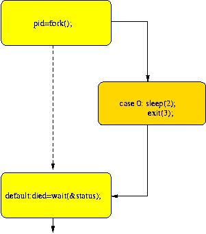
Unix Fork

from
http://www.eng.cam.ac.uk/help/tpl/unix/fork.html

#include
#include
#include
using namespace std;
int main(){
pid_t pid;
int status, died;
switch(pid=fork()){
case -1: cout << "can't fork\n";
exit(-1);
case 0 : sleep(2); // this is the code the child runs
exit(3);
default: died= wait(&status); // this is the code the parent runs
}
}

Good Site for Design Patterns

http://home.earthlink.net/~huston2/dp/FactoryDemosCpp

Singleton Pattern in C++

from devx.com site

Implementing the Singleton Design Pattern
By Danny Kalev

Singleton is probably the most widely used design pattern. Its intent is to ensure that a class has only one instance, and to provide a global point of access to it. There are many situations in which a singleton object is necessary: a GUI application must have a single mouse, an active modem needs one and only one telephone line, an operating system can only have one window manager, and a PC is connected to a single keyboard. I will show how to implement the singleton pattern in C++ and explain how you can optimize its design for single-threaded applications.

Design Considerations
Using a global object ensures that the instance is easily accessible but it doesn't keep you from instantiating multiple objects—you can still create a local instance of the same class in addition to the global one. The Singleton pattern provides an elegant solution to this problem by making the class itself responsible for managing its sole instance. The sole instance is an ordinary object of its class, but that class is written so that only one instance can ever be created. This way, you guarantee that no other instance can be created. Furthermore, you provide a global point of access to that instance. The Singleton class hides the operation that creates the instance behind a static member function. This member function, traditionally called Instance(), returns a pointer to the sole instance. Here's a declaration of such a class:


class Singleton
{
public:
static Singleton* Instance();
protected:
Singleton();
Singleton(const Singleton&);
Singleton& operator= (const Singleton&);
private:
static Singleton* pinstance;
};

Instead of Singleton, you can name your class Mouse, FileManager, Scheduler, etc., and declare additional members accordingly. To ensure that users can't create local instances of the class, Singleton's constructor, assignment operator, and copy constructor are declared protected. The class also declares a private static pointer to its instance, pinstance. When the static function Instance() is called for the first time, it creates the sole instance, assigns its address to pinstance, and returns that address. In every subsequent invocation, Instance() will merely return that address.

The class's implementation looks like this:


Singleton* Singleton::pinstance = 0;// initialize pointer
Singleton* Singleton::Instance ()
{
if (pinstance == 0) // is it the first call?
{
pinstance = new Singleton; // create sole instance
}
return pinstance; // address of sole instance
}
Singleton::Singleton()
{
//... perform necessary instance initializations
}

Users access the sole instance through the Instance() member function exclusively. Any attempt to create an instance not through this function will fail because the class's constructor is protected. Instance() uses lazy initialization. This means the value it returns is created when the function is accessed for the first time. Note that this design is bullet-proof—all the following Instance() calls return a pointer to the same instance:


Singleton *p1 = Singleton::Instance();
Singleton *p2 = p1->Instance();
Singleton & ref = * Singleton::Instance();

Although our example uses a single instance, with minor modifications to the function Instance(), this design pattern permits a variable number of instances. For example, you can design a class that allows up to five instances.

Optimizing Singleton for Single-Threaded Applications
Singleton allocates its sole instance on the free-store using operator new. Because operator new is thread-safe, you can use this design pattern in multi-threaded applications. However, there's a fly in the ointment: you must destroy the instance manually by calling delete before the application terminates. Otherwise, not only are you causing a memory leak, but you also bring about undefined behavior because Singleton's destructor will never get called. Single-threaded applications can easily avoid this hassle by using a local static instance instead of a dynamically allocated one. Here's a slightly different implementation of Instance() that's suitable for single-threaded applications:


Singleton* Singleton::Instance ()
{
static Singleton inst;
return &inst;
}

The local static object inst is constructed when Instance() is called for the first time and remains alive until the application terminates. Note that the pointer pinstance is now redundant and can be removed from the class's declaration. Unlike dynamically allocated objects, static objects are destroyed automatically when the application terminates, so you shouldn't destroy the instance manually.

Constant Pointers in C++

Fromm C++ faq lite

What's the difference between "const Fred* p", "Fred* const p" and "const Fred* const p"?

You have to read pointer declarations right-to-left.

* const Fred* p means "p points to a Fred that is const" — that is, the Fred object can't be changed via p.
* Fred* const p means "p is a const pointer to a Fred" — that is, you can change the Fred object via p, but you can't change the pointer p itself.
* const Fred* const p means "p is a const pointer to a const Fred" — that is, you can't change the pointer p itself, nor can you change the Fred object via p.

Normal Forms Again

From Google

1 INTRODUCTION

The normal forms defined in relational database theory represent guidelines for record design. The guidelines corresponding to first through fifth normal forms are presented here, in terms that do not require an understanding of relational theory. The design guidelines are meaningful even if one is not using a relational database system. We present the guidelines without referring to the concepts of the relational model in order to emphasize their generality, and also to make them easier to understand. Our presentation conveys an intuitive sense of the intended constraints on record design, although in its informality it may be imprecise in some technical details. A comprehensive treatment of the subject is provided by Date [4].

The normalization rules are designed to prevent update anomalies and data inconsistencies. With respect to performance tradeoffs, these guidelines are biased toward the assumption that all non-key fields will be updated frequently. They tend to penalize retrieval, since data which may have been retrievable from one record in an unnormalized design may have to be retrieved from several records in the normalized form. There is no obligation to fully normalize all records when actual performance requirements are taken into account.
2 FIRST NORMAL FORM

First normal form [1] deals with the "shape" of a record type.

Under first normal form, all occurrences of a record type must contain the same number of fields.

First normal form excludes variable repeating fields and groups. This is not so much a design guideline as a matter of definition. Relational database theory doesn't deal with records having a variable number of fields.
3 SECOND AND THIRD NORMAL FORMS

Second and third normal forms [2, 3, 7] deal with the relationship between non-key and key fields.

Under second and third normal forms, a non-key field must provide a fact about the key, us the whole key, and nothing but the key. In addition, the record must satisfy first normal form.

We deal now only with "single-valued" facts. The fact could be a one-to-many relationship, such as the department of an employee, or a one-to-one relationship, such as the spouse of an employee. Thus the phrase "Y is a fact about X" signifies a one-to-one or one-to-many relationship between Y and X. In the general case, Y might consist of one or more fields, and so might X. In the following example, QUANTITY is a fact about the combination of PART and WAREHOUSE.
3.1 Second Normal Form

Second normal form is violated when a non-key field is a fact about a subset of a key. It is only relevant when the key is composite, i.e., consists of several fields. Consider the following inventory record:

---------------------------------------------------
| PART | WAREHOUSE | QUANTITY | WAREHOUSE-ADDRESS |
====================-------------------------------

The key here consists of the PART and WAREHOUSE fields together, but WAREHOUSE-ADDRESS is a fact about the WAREHOUSE alone. The basic problems with this design are:

* The warehouse address is repeated in every record that refers to a part stored in that warehouse.
* If the address of the warehouse changes, every record referring to a part stored in that warehouse must be updated.
* Because of the redundancy, the data might become inconsistent, with different records showing different addresses for the same warehouse.
* If at some point in time there are no parts stored in the warehouse, there may be no record in which to keep the warehouse's address.

To satisfy second normal form, the record shown above should be decomposed into (replaced by) the two records:

------------------------------- ---------------------------------
| PART | WAREHOUSE | QUANTITY | | WAREHOUSE | WAREHOUSE-ADDRESS |
====================----------- =============--------------------

When a data design is changed in this way, replacing unnormalized records with normalized records, the process is referred to as normalization. The term "normalization" is sometimes used relative to a particular normal form. Thus a set of records may be normalized with respect to second normal form but not with respect to third.

The normalized design enhances the integrity of the data, by minimizing redundancy and inconsistency, but at some possible performance cost for certain retrieval applications. Consider an application that wants the addresses of all warehouses stocking a certain part. In the unnormalized form, the application searches one record type. With the normalized design, the application has to search two record types, and connect the appropriate pairs.
3.2 Third Normal Form

Third normal form is violated when a non-key field is a fact about another non-key field, as in

------------------------------------
| EMPLOYEE | DEPARTMENT | LOCATION |
============------------------------

The EMPLOYEE field is the key. If each department is located in one place, then the LOCATION field is a fact about the DEPARTMENT -- in addition to being a fact about the EMPLOYEE. The problems with this design are the same as those caused by violations of second normal form:

* The department's location is repeated in the record of every employee assigned to that department.
* If the location of the department changes, every such record must be updated.
* Because of the redundancy, the data might become inconsistent, with different records showing different locations for the same department.
* If a department has no employees, there may be no record in which to keep the department's location.

To satisfy third normal form, the record shown above should be decomposed into the two records:

------------------------- -------------------------
| EMPLOYEE | DEPARTMENT | | DEPARTMENT | LOCATION |
============------------- ==============-----------

To summarize, a record is in second and third normal forms if every field is either part of the key or provides a (single-valued) fact about exactly the whole key and nothing else.

SQL Server Impersonation Error While Deploying Models

http://forums.microsoft.com/MSDN/ShowPost.aspx?PostID=148964&SiteID=1

SQL Server 2005 Key Columns

Specifying the Column Usage

After you specify the case table and the nested tables, you determine the usage type for each column in the tables that you will include in the mining structure. If you do not specify a usage type for a column, the column will not be included in the mining structure. Data mining columns can be one of four types: key, input, predictable, or a combination of input and predictable. Key columns contain a unique identifier for each row in a table. Some mining models, such as sequence clustering and time series models, can contain multiple key columns. Input columns provide the information from which predictions are made. Predictable columns contain the information that you try to predict in the mining model.

For example, a series of tables may contain customer IDs, demographic information, and the amount of money each customer spends at a specific store. The customer ID uniquely identifies the customer and also relates the case table to the nested tables, therefore you would use it as the key column. You could use a selection of columns from the demographic information as input columns, and the column that describes the amount of money each customer spends as a predictable column. You could then build a mining model that relates demographics to how much money a customer spends in a store. You could use this model as the basis for targeted marketing.

The Data Mining Wizard provides the Suggest feature, which is enabled when you select a predictable column. Datasets frequently contain more columns than you want to use to build a mining model. The Suggest feature calculates a numeric score, from 0 to 1, that describes the relationship between each column in the dataset and the predictable column. Based on this score, the feature suggests columns to use as input for the mining model. If you use the Suggest feature, you can use the suggested columns, modify the selections to fit your needs, or ignore the suggestions.
Specifying the Content and Data Types

After you select one or more predictable columns and input columns, you can specify the content and data types for each column.

Nested and Case Tables

Stolen from Microsoft
http://msdn2.microsoft.com/en-us/library/ms175659.aspx

Nested Tables

In Microsoft SQL Server 2005 Analysis Services (SSAS), data must be fed to a data mining algorithm as a series of cases that are contained within a case table. Not all cases can be described by a single row of data. For example, a case may be derived from two tables, one table that contains customer information and another table that contains customer purchases. A single customer in the customer table may have multiple purchases in the purchases table, which makes it difficult to describe the data using a single row. Analysis Services provides a unique method for handling these cases, by using nested tables. The concept of a nested table is demonstrated in the following illustration.
Two tables combined by using a nested table

In this diagram, the first table, which is the parent table, contains information about customers, and associates a unique identifier for each customer. The second table, the child table, contains purchases for each customer. The purchases in the child table are related back to the parent table by the unique identifier, the CustomerKey column. The third table in the diagram shows the two tables combined.

A nested table is represented in the case table as a special column that has a data type of TABLE. For any particular case row, this kind of column contains selected rows from the child table that pertain to the parent table.

In order to create a nested table, the two source tables must contain a defined relationship so that the items in one table can be related back to the other table. In Business Intelligence Development Studio, you can define this relationship within the data source view. For more information about how to define a relationship between two tables, see How to: Add a Relationship Between Two Tables Using the Data Source View Designer.

You can create nested tables programmatically by either using Data Mining Extensions (DMX) or Analysis Management Objects (AMO), or you can use the Data Mining Wizard and Data Mining Designer in Business Intelligence Development Studio.