Friday, March 10, 2006

Unix Fork


from
http://www.eng.cam.ac.uk/help/tpl/unix/fork.html

#include
#include
#include
using namespace std;
int main(){
pid_t pid;
int status, died;
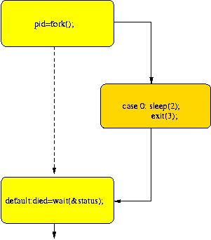
switch(pid=fork()){
case -1: cout << "can't fork\n";
exit(-1);
case 0 : sleep(2); // this is the code the child runs
exit(3);
default: died= wait(&status); // this is the code the parent runs
}
}

Thursday, March 09, 2006

Good Site for Design Patterns

http://home.earthlink.net/~huston2/dp/FactoryDemosCpp

Singleton Pattern in C++

from devx.com site

Implementing the Singleton Design Pattern
By Danny Kalev

Singleton is probably the most widely used design pattern. Its intent is to ensure that a class has only one instance, and to provide a global point of access to it. There are many situations in which a singleton object is necessary: a GUI application must have a single mouse, an active modem needs one and only one telephone line, an operating system can only have one window manager, and a PC is connected to a single keyboard. I will show how to implement the singleton pattern in C++ and explain how you can optimize its design for single-threaded applications.

Design Considerations
Using a global object ensures that the instance is easily accessible but it doesn't keep you from instantiating multiple objects—you can still create a local instance of the same class in addition to the global one. The Singleton pattern provides an elegant solution to this problem by making the class itself responsible for managing its sole instance. The sole instance is an ordinary object of its class, but that class is written so that only one instance can ever be created. This way, you guarantee that no other instance can be created. Furthermore, you provide a global point of access to that instance. The Singleton class hides the operation that creates the instance behind a static member function. This member function, traditionally called Instance(), returns a pointer to the sole instance. Here's a declaration of such a class:


class Singleton
{
public:
static Singleton* Instance();
protected:
Singleton();
Singleton(const Singleton&);
Singleton& operator= (const Singleton&);
private:
static Singleton* pinstance;
};

Instead of Singleton, you can name your class Mouse, FileManager, Scheduler, etc., and declare additional members accordingly. To ensure that users can't create local instances of the class, Singleton's constructor, assignment operator, and copy constructor are declared protected. The class also declares a private static pointer to its instance, pinstance. When the static function Instance() is called for the first time, it creates the sole instance, assigns its address to pinstance, and returns that address. In every subsequent invocation, Instance() will merely return that address.

The class's implementation looks like this:


Singleton* Singleton::pinstance = 0;// initialize pointer
Singleton* Singleton::Instance ()
{
if (pinstance == 0) // is it the first call?
{
pinstance = new Singleton; // create sole instance
}
return pinstance; // address of sole instance
}
Singleton::Singleton()
{
//... perform necessary instance initializations
}

Users access the sole instance through the Instance() member function exclusively. Any attempt to create an instance not through this function will fail because the class's constructor is protected. Instance() uses lazy initialization. This means the value it returns is created when the function is accessed for the first time. Note that this design is bullet-proof—all the following Instance() calls return a pointer to the same instance:


Singleton *p1 = Singleton::Instance();
Singleton *p2 = p1->Instance();
Singleton & ref = * Singleton::Instance();

Although our example uses a single instance, with minor modifications to the function Instance(), this design pattern permits a variable number of instances. For example, you can design a class that allows up to five instances.

Optimizing Singleton for Single-Threaded Applications
Singleton allocates its sole instance on the free-store using operator new. Because operator new is thread-safe, you can use this design pattern in multi-threaded applications. However, there's a fly in the ointment: you must destroy the instance manually by calling delete before the application terminates. Otherwise, not only are you causing a memory leak, but you also bring about undefined behavior because Singleton's destructor will never get called. Single-threaded applications can easily avoid this hassle by using a local static instance instead of a dynamically allocated one. Here's a slightly different implementation of Instance() that's suitable for single-threaded applications:


Singleton* Singleton::Instance ()
{
static Singleton inst;
return &inst;
}

The local static object inst is constructed when Instance() is called for the first time and remains alive until the application terminates. Note that the pointer pinstance is now redundant and can be removed from the class's declaration. Unlike dynamically allocated objects, static objects are destroyed automatically when the application terminates, so you shouldn't destroy the instance manually.

Wednesday, March 08, 2006

Constant Pointers in C++

Fromm C++ faq lite

What's the difference between "const Fred* p", "Fred* const p" and "const Fred* const p"?

You have to read pointer declarations right-to-left.

* const Fred* p means "p points to a Fred that is const" — that is, the Fred object can't be changed via p.
* Fred* const p means "p is a const pointer to a Fred" — that is, you can change the Fred object via p, but you can't change the pointer p itself.
* const Fred* const p means "p is a const pointer to a const Fred" — that is, you can't change the pointer p itself, nor can you change the Fred object via p.

Monday, March 06, 2006

Normal Forms Again

From Google

1 INTRODUCTION

The normal forms defined in relational database theory represent guidelines for record design. The guidelines corresponding to first through fifth normal forms are presented here, in terms that do not require an understanding of relational theory. The design guidelines are meaningful even if one is not using a relational database system. We present the guidelines without referring to the concepts of the relational model in order to emphasize their generality, and also to make them easier to understand. Our presentation conveys an intuitive sense of the intended constraints on record design, although in its informality it may be imprecise in some technical details. A comprehensive treatment of the subject is provided by Date [4].

The normalization rules are designed to prevent update anomalies and data inconsistencies. With respect to performance tradeoffs, these guidelines are biased toward the assumption that all non-key fields will be updated frequently. They tend to penalize retrieval, since data which may have been retrievable from one record in an unnormalized design may have to be retrieved from several records in the normalized form. There is no obligation to fully normalize all records when actual performance requirements are taken into account.
2 FIRST NORMAL FORM

First normal form [1] deals with the "shape" of a record type.

Under first normal form, all occurrences of a record type must contain the same number of fields.

First normal form excludes variable repeating fields and groups. This is not so much a design guideline as a matter of definition. Relational database theory doesn't deal with records having a variable number of fields.
3 SECOND AND THIRD NORMAL FORMS

Second and third normal forms [2, 3, 7] deal with the relationship between non-key and key fields.

Under second and third normal forms, a non-key field must provide a fact about the key, us the whole key, and nothing but the key. In addition, the record must satisfy first normal form.

We deal now only with "single-valued" facts. The fact could be a one-to-many relationship, such as the department of an employee, or a one-to-one relationship, such as the spouse of an employee. Thus the phrase "Y is a fact about X" signifies a one-to-one or one-to-many relationship between Y and X. In the general case, Y might consist of one or more fields, and so might X. In the following example, QUANTITY is a fact about the combination of PART and WAREHOUSE.
3.1 Second Normal Form

Second normal form is violated when a non-key field is a fact about a subset of a key. It is only relevant when the key is composite, i.e., consists of several fields. Consider the following inventory record:

---------------------------------------------------
| PART | WAREHOUSE | QUANTITY | WAREHOUSE-ADDRESS |
====================-------------------------------

The key here consists of the PART and WAREHOUSE fields together, but WAREHOUSE-ADDRESS is a fact about the WAREHOUSE alone. The basic problems with this design are:

* The warehouse address is repeated in every record that refers to a part stored in that warehouse.
* If the address of the warehouse changes, every record referring to a part stored in that warehouse must be updated.
* Because of the redundancy, the data might become inconsistent, with different records showing different addresses for the same warehouse.
* If at some point in time there are no parts stored in the warehouse, there may be no record in which to keep the warehouse's address.

To satisfy second normal form, the record shown above should be decomposed into (replaced by) the two records:

------------------------------- ---------------------------------
| PART | WAREHOUSE | QUANTITY | | WAREHOUSE | WAREHOUSE-ADDRESS |
====================----------- =============--------------------

When a data design is changed in this way, replacing unnormalized records with normalized records, the process is referred to as normalization. The term "normalization" is sometimes used relative to a particular normal form. Thus a set of records may be normalized with respect to second normal form but not with respect to third.

The normalized design enhances the integrity of the data, by minimizing redundancy and inconsistency, but at some possible performance cost for certain retrieval applications. Consider an application that wants the addresses of all warehouses stocking a certain part. In the unnormalized form, the application searches one record type. With the normalized design, the application has to search two record types, and connect the appropriate pairs.
3.2 Third Normal Form

Third normal form is violated when a non-key field is a fact about another non-key field, as in

------------------------------------
| EMPLOYEE | DEPARTMENT | LOCATION |
============------------------------

The EMPLOYEE field is the key. If each department is located in one place, then the LOCATION field is a fact about the DEPARTMENT -- in addition to being a fact about the EMPLOYEE. The problems with this design are the same as those caused by violations of second normal form:

* The department's location is repeated in the record of every employee assigned to that department.
* If the location of the department changes, every such record must be updated.
* Because of the redundancy, the data might become inconsistent, with different records showing different locations for the same department.
* If a department has no employees, there may be no record in which to keep the department's location.

To satisfy third normal form, the record shown above should be decomposed into the two records:

------------------------- -------------------------
| EMPLOYEE | DEPARTMENT | | DEPARTMENT | LOCATION |
============------------- ==============-----------

To summarize, a record is in second and third normal forms if every field is either part of the key or provides a (single-valued) fact about exactly the whole key and nothing else.

Saturday, March 04, 2006

SQL Server Impersonation Error While Deploying Models

http://forums.microsoft.com/MSDN/ShowPost.aspx?PostID=148964&SiteID=1

Friday, March 03, 2006

SQL Server 2005 Key Columns

Specifying the Column Usage

After you specify the case table and the nested tables, you determine the usage type for each column in the tables that you will include in the mining structure. If you do not specify a usage type for a column, the column will not be included in the mining structure. Data mining columns can be one of four types: key, input, predictable, or a combination of input and predictable. Key columns contain a unique identifier for each row in a table. Some mining models, such as sequence clustering and time series models, can contain multiple key columns. Input columns provide the information from which predictions are made. Predictable columns contain the information that you try to predict in the mining model.

For example, a series of tables may contain customer IDs, demographic information, and the amount of money each customer spends at a specific store. The customer ID uniquely identifies the customer and also relates the case table to the nested tables, therefore you would use it as the key column. You could use a selection of columns from the demographic information as input columns, and the column that describes the amount of money each customer spends as a predictable column. You could then build a mining model that relates demographics to how much money a customer spends in a store. You could use this model as the basis for targeted marketing.

The Data Mining Wizard provides the Suggest feature, which is enabled when you select a predictable column. Datasets frequently contain more columns than you want to use to build a mining model. The Suggest feature calculates a numeric score, from 0 to 1, that describes the relationship between each column in the dataset and the predictable column. Based on this score, the feature suggests columns to use as input for the mining model. If you use the Suggest feature, you can use the suggested columns, modify the selections to fit your needs, or ignore the suggestions.
Specifying the Content and Data Types

After you select one or more predictable columns and input columns, you can specify the content and data types for each column.

Nested and Case Tables

Stolen from Microsoft
http://msdn2.microsoft.com/en-us/library/ms175659.aspx

Nested Tables

In Microsoft SQL Server 2005 Analysis Services (SSAS), data must be fed to a data mining algorithm as a series of cases that are contained within a case table. Not all cases can be described by a single row of data. For example, a case may be derived from two tables, one table that contains customer information and another table that contains customer purchases. A single customer in the customer table may have multiple purchases in the purchases table, which makes it difficult to describe the data using a single row. Analysis Services provides a unique method for handling these cases, by using nested tables. The concept of a nested table is demonstrated in the following illustration.
Two tables combined by using a nested table

In this diagram, the first table, which is the parent table, contains information about customers, and associates a unique identifier for each customer. The second table, the child table, contains purchases for each customer. The purchases in the child table are related back to the parent table by the unique identifier, the CustomerKey column. The third table in the diagram shows the two tables combined.

A nested table is represented in the case table as a special column that has a data type of TABLE. For any particular case row, this kind of column contains selected rows from the child table that pertain to the parent table.

In order to create a nested table, the two source tables must contain a defined relationship so that the items in one table can be related back to the other table. In Business Intelligence Development Studio, you can define this relationship within the data source view. For more information about how to define a relationship between two tables, see How to: Add a Relationship Between Two Tables Using the Data Source View Designer.

You can create nested tables programmatically by either using Data Mining Extensions (DMX) or Analysis Management Objects (AMO), or you can use the Data Mining Wizard and Data Mining Designer in Business Intelligence Development Studio.

Thursday, February 23, 2006

Outer Product

Outer Product

The outer product is a way to build a higher rank tensor from those of lower rank. . One use of this is to combine two vectors to form a matrix as an outer product.
vec1 = {a,b,c}
vec2 = {x,y,z}

Inner product (dot product which would result in a scalar) = vec1 * vec2'

= {a,b,c} * { x} = ax + by + cz
{ y}
{ z}

Whereas the outerproduct is to increase the rank = vec1' * vec2

= {a} * { x, y, z} =
{b}
{c}

= ax, ay, az
bx, by, bz
cx, cy, cz

Monday, January 16, 2006

EM

1. A good reference is the Tom Mitchell: Machine learning, A gentle tutorial on EM algorithm.

2. What is a mixture model?
Stolen from Wikipedia

A mixture model is a model in which the independent variables are measured as fractions of a total. For example, suppose researchers are trying to find the optimal mixture of ingredients for a fruit punch consisting of grape juice, mango juice, and pineapple juice. A mixture model is suitable here because the results of the taste tests will not depend on the amount of ingredients used to make the batch but rather on the fraction of each ingredient present in the punch. The sum of the mixture components is always 100%, and a mixture model takes this restriction into account.

[edit]
Another definition
A mixture model can also be a formalism for modeling a probability density function as a sum of parameterized functions. In mathematical terms,


where pX(x) is the modeled probability distribution function, K is the number of components in the mixture model, and ak is mixture proportion of component k. By definition, 0 < ak < 1 for all and .

h(x | λk) is a probability distribution parameterized by λk.
Mixture models are often used when we know h(x) and we can sample from pX(x), but we would like to determine the ak and λk values. Such situations can arise in studies in which we sample from a population that is composed of several distinct subpopulations.

[edit]
Two common approaches for estimation in mixture models
It's common to think of mixture modeling (under the second definition) as a missing data problem. One way to understand this is to assume that the data points under consideration have "membership" in one of the distributions we are using to model the data. When we start, this membership is unknown, or missing. The job of estimation is to devise appropriate parameters for the model functions we choose, with the connection to the data points being represented as their membership in the individual model distributions.

[edit]
Expectation maximization
The Expectation-maximization algorithm is one way to compute the missing memberships of data points in our chosen distribution model. It is an iterative procedure, where we start with initial parameters for our model distribution (the ak's and λk's of the model listed above). The estimation process proceeds iteratively in two steps, the Expectation Step, and the Maximization Step.

[edit]
The expectation step
With initial guesses for the parameters in our mixture model, we compute "partial membership" of each data point in each constituent distribution. This is done by calculating expectation values for the membership variables of each data point. An example will provide some clarity. Let's consider a simple example. We have a collection of data points xi that can be modeled as coming from a sum of two Gaussian distributions. The probability expression for our model is


Where f is the mixing coefficient in [0,1] (ak = 2 = f and ak = 1 = 1 − f), and we assume σ is known and constant. For each of our data points xi, we can compute a membership value for each of the two Gaussians as follows


and similarly for y2,i.

In the case of a Gaussian mixture model,


[edit]
The maximization step
With our expectation values in hand for group membership, we can recompute plug-in estimates of our distribution parameters. For the mixing coefficient f this is simply the fractional membership of all data points in the second Gaussian.


where N is the total number of data points. For μ1,


With new estimates for f and the μ's, we proceed back to the Expectation step to recompute new membership values. The procedure is repeated until there is no further change in the mixture model parameters.

Saturday, January 07, 2006

Java Operators

* << left-shift, >> right-shift, >>> unsigned right-shift
* only used on integer values
* binary numeric promotion is not performed on the operands; instead unary promotion is performed on each operand separately (JLS §15.19)
* both operands are individually promoted to int if their type is byte, short or char
* a long shift operator does not force a left-hand int value promotion to long (JLS§5.6.1)
* left-associative
* left-hand operator represents the number to be shifted
* right-hand operator specifies the shift distance

value << 2 // 2 is the distance to be shifted

* when the value to be shifted (left-operand) is an int, only the last 5 digits of the right-hand operand are used to perform the shift. The actual size of the shift is the value of the right-hand operand masked by 31 (0x1f). ie the shift distance is always between 0 and 31 (if shift value is > 32 shift is 32%value)

35 00000000 00000000 00000000 00100011
31 -> 0x1f 00000000 00000000 00000000 00011111
& -----------------------------------
Shift value 00000000 00000000 00000000 00000011 -> 3

-29 11111111 11111111 11111111 11100011
31 -> 0x1f 00000000 00000000 00000000 00011111
& -----------------------------------
Shift value 00000000 00000000 00000000 00000011 -> 3

* when the value to be shifted (left-operand) is a long, only the last 6 digits of the right-hand operand are used to perform the shift. The actual size of the shift is the value of the right-hand operand masked by 63 (0x3D) ie the shift distance is always between 0 and 63 (if shift value is greater than 64 shift is 64%value)
* the shift occurs at runtime on a bit-by-bit basis

Left-shift << (JLS §15.19)

* bits are shifted to the left based on the value of the right-operand
* new right hand bits are zero filled
* equivalent to left-operand times two to the power of the right-operand
For example, 16 << 5 = 16 * 25 = 512

Decimal 16 00000000000000000000000000010000

Left-shift 5 00000000000000000000000000010000
fill right 0000000000000000000000000001000000000
discard left 00000000000000000000001000000000

* the sign-bit is shifted to the left as well, so it can be dropped off or a different sign can replace it

Right-shift >> (JLS §15.19)

* bits are shifted to the right based on value of right-operand
* new left hand bits are filled with the value of the left-operand high-order bit therefore the sign of the left-hand operator is always retained
* for non-negative integers, a right-shift is equivalent to dividing the left-hand operator by two to the power of the right-hand operator
For example: 16 >> 2 = 16 / 22 = 4

Decimal 16 00000000000000000000000000010000

Right-shift 2 00000000000000000000000000010000
fill left 00000000000000000000000000000100
discard right 00000000000000000000000000000100 -> Decimal 4

Decimal -16 11111111111111111111111111110000

Right-shift 2 11111111111111111111111111110000
fill left 1111111111111111111111111111110000
discard right 11111111111111111111111111111100 -> Decimal -4

Unsigned right-shift >>> (JLS §15.19)

* identical to the right-shift operator only the left-bits are zero filled
* because the left-operand high-order bit is not retained, the sign value can change
* if the left-hand operand is positive, the result is the same as a right-shift
* if the left-hand operand is negative, the result is equivalent to the left-hand operand right-shifted by the number indicated by the right-hand operand plus two left-shifted by the inverted value of the right-hand operand
For example: -16 >>> 2 = (-16 >> 2 ) + ( 2 << ~2 ) = 1,073,741,820

Decimal 16 00000000000000000000000000010000

Right-shift 2 00000000000000000000000000010000
fill left 00000000000000000000000000000100
discard right 00000000000000000000000000000100 -> Decimal 4

Decimal -16 11111111111111111111111111110000

>>> 2 11111111111111111111111111110000
fill left 0011111111111111111111111111110000
discard right 00111111111111111111111111111100

Gaussian Mixture Models

Gaussian Mixture Models are universal approximators of densities.
Gaussian Mixture Models are trained by maximum likelihood using Expectation Maximization algorithm

Friday, January 06, 2006

Oracle DBA Interview Question

from databasejournal.com(James Koopmann)

1. Explain the difference between a hot backup and a cold backup and the benefits associated with each.

A hot backup is basically taking a backup of the database while it is still up and running and it must be in archive log mode. A cold backup is taking a backup of the database while it is shut down and does not require being in archive log mode. The benefit of taking a hot backup is that the database is still available for use while the backup is occurring and you can recover the database to any point in time. The benefit of taking a cold backup is that it is typically easier to administer the backup and recovery process. In addition, since you are taking cold backups the database does not require being in archive log mode and thus there will be a slight performance gain as the database is not cutting archive logs to disk.

2. You have just had to restore from backup and do not have any control files. How would you go about bringing up this database?

I would create a text based backup control file, stipulating where on disk all the data files where and then issue the recover command with the using backup control file clause.

3. How do you switch from an init.ora file to a spfile?

Issue the create spfile from pfile command.

4. Explain the difference between a data block, an extent and a segment.

A data block is the smallest unit of logical storage for a database object. As objects grow they take chunks of additional storage that are composed of contiguous data blocks. These groupings of contiguous data blocks are called extents. All the extents that an object takes when grouped together are considered the segment of the database object.

5. Give two examples of how you might determine the structure of the table DEPT.

Use the describe command or use the dbms_metadata.get_ddl package.

6. Where would you look for errors from the database engine?

In the alert log.

7. Compare and contrast TRUNCATE and DELETE for a table.

Both the truncate and delete command have the desired outcome of getting rid of all the rows in a table. The difference between the two is that the truncate command is a DDL operation and just moves the high water mark and produces a now rollback. The delete command, on the other hand, is a DML operation, which will produce a rollback and thus take longer to complete.

8. Give the reasoning behind using an index.

Faster access to data blocks in a table.

9. Give the two types of tables involved in producing a star schema and the type of data they hold.

Fact tables and dimension tables. A fact table contains measurements while dimension tables will contain data that will help describe the fact tables.

10. . What type of index should you use on a fact table?

A Bitmap index.

11. Give two examples of referential integrity constraints.

A primary key and a foreign key.

12. A table is classified as a parent table and you want to drop and re-create it. How would you do this without affecting the children tables?

Disable the foreign key constraint to the parent, drop the table, re-create the table, enable the foreign key constraint.

13. Explain the difference between ARCHIVELOG mode and NOARCHIVELOG mode and the benefits and disadvantages to each.

ARCHIVELOG mode is a mode that you can put the database in for creating a backup of all transactions that have occurred in the database so that you can recover to any point in time. NOARCHIVELOG mode is basically the absence of ARCHIVELOG mode and has the disadvantage of not being able to recover to any point in time. NOARCHIVELOG mode does have the advantage of not having to write transactions to an archive log and thus increases the performance of the database slightly.

14. What command would you use to create a backup control file?

Alter database backup control file to trace.

15. Give the stages of instance startup to a usable state where normal users may access it.

STARTUP NOMOUNT - Instance startup

STARTUP MOUNT - The database is mounted

STARTUP OPEN - The database is opened

16. What column differentiates the V$ views to the GV$ views and how?

The INST_ID column which indicates the instance in a RAC environment the information came from.

17. How would you go about generating an EXPLAIN plan?

Create a plan table with utlxplan.sql.

Use the explain plan set statement_id = 'tst1' into plan_table for a SQL statement

Look at the explain plan with utlxplp.sql or utlxpls.sql

18. How would you go about increasing the buffer cache hit ratio?

Use the buffer cache advisory over a given workload and then query the v$db_cache_advice table. If a change was necessary then I would use the alter system set db_cache_size command.

19. Explain an ORA-01555

You get this error when you get a snapshot too old within rollback. It can usually be solved by increasing the undo retention or increasing the size of rollbacks. You should also look at the logic involved in the application getting the error message.

20. Explain the difference between $ORACLE_HOME and $ORACLE_BASE.

ORACLE_BASE is the root directory for oracle. ORACLE_HOME located beneath ORACLE_BASE is where the oracle products reside.

21. How would you determine the time zone under which a database was operating?

select DBTIMEZONE from dual;

22. Explain the use of setting GLOBAL_NAMES equal to TRUE.

Setting GLOBAL_NAMES dictates how you might connect to a database. This variable is either TRUE or FALSE and if it is set to TRUE it enforces database links to have the same name as the remote database to which they are linking.

23. What command would you use to encrypt a PL/SQL application?

WRAP

24. Explain the difference between a FUNCTION, PROCEDURE and PACKAGE.

A function and procedure are the same in that they are intended to be a collection of PL/SQL code that carries a single task. While a procedure does not have to return any values to the calling application, a function will return a single value. A package on the other hand is a collection of functions and procedures that are grouped together based on their commonality to a business function or application.

25. Explain the use of table functions.

Table functions are designed to return a set of rows through PL/SQL logic but are intended to be used as a normal table or view in a SQL statement. They are also used to pipeline information in an ETL process.

26. Name three advisory statistics you can collect.

Buffer Cache Advice, Segment Level Statistics, & Timed Statistics

27. Where in the Oracle directory tree structure are audit traces placed?

In unix $ORACLE_HOME/rdbms/audit, in Windows the event viewer

28. Explain materialized views and how they are used.

Materialized views are objects that are reduced sets of information that have been summarized, grouped, or aggregated from base tables. They are typically used in data warehouse or decision support systems.

29. When a user process fails, what background process cleans up after it?

PMON

30. What background process refreshes materialized views?

The Job Queue Processes.

31. How would you determine what sessions are connected and what resources they are waiting for?

Use of V$SESSION and V$SESSION_WAIT

32. Describe what redo logs are.

Redo logs are logical and physical structures that are designed to hold all the changes made to a database and are intended to aid in the recovery of a database.

33. How would you force a log switch?

ALTER SYSTEM SWITCH LOGFILE;

34. Give two methods you could use to determine what DDL changes have been made.

You could use Logminer or Streams

35. What does coalescing a tablespace do?

Coalescing is only valid for dictionary-managed tablespaces and de-fragments space by combining neighboring free extents into large single extents.

36. What is the difference between a TEMPORARY tablespace and a PERMANENT tablespace?

A temporary tablespace is used for temporary objects such as sort structures while permanent tablespaces are used to store those objects meant to be used as the true objects of the database.

37. Name a tablespace automatically created when you create a database.

The SYSTEM tablespace.

38. When creating a user, what permissions must you grant to allow them to connect to the database?

Grant the CONNECT to the user.

39. How do you add a data file to a tablespace?

ALTER TABLESPACE ADD DATAFILE SIZE

40. How do you resize a data file?

ALTER DATABASE DATAFILE RESIZE ;

41. What view would you use to look at the size of a data file?

DBA_DATA_FILES

42. What view would you use to determine free space in a tablespace?

DBA_FREE_SPACE

43. How would you determine who has added a row to a table?

Turn on fine grain auditing for the table.

44. How can you rebuild an index?

ALTER INDEX REBUILD;

45. Explain what partitioning is and what its benefit is.

Partitioning is a method of taking large tables and indexes and splitting them into smaller, more manageable pieces.

46. You have just compiled a PL/SQL package but got errors, how would you view the errors?

SHOW ERRORS

47. How can you gather statistics on a table?

The ANALYZE command.

48. How can you enable a trace for a session?

Use the DBMS_SESSION.SET_SQL_TRACE or

Use ALTER SESSION SET SQL_TRACE = TRUE;

49. What is the difference between the SQL*Loader and IMPORT utilities?

These two Oracle utilities are used for loading data into the database. The difference is that the import utility relies on the data being produced by another Oracle utility EXPORT while the SQL*Loader utility allows data to be loaded that has been produced by other utilities from different data sources just so long as it conforms to ASCII formatted or delimited files.

50. Name two files used for network connection to a database.

TNSNAMES.ORA and SQLNET.ORA
Technical - UNIX

Every DBA should know something about the operating system that the database will be running on. The questions here are related to UNIX but you should equally be able to answer questions related to common Windows environments.

1. How do you list the files in an UNIX directory while also showing hidden files?

ls -ltra

2. How do you execute a UNIX command in the background?

Use the "&"

3. What UNIX command will control the default file permissions when files are created?

Umask

4. Explain the read, write, and execute permissions on a UNIX directory.

Read allows you to see and list the directory contents.

Write allows you to create, edit and delete files and subdirectories in the directory.

Execute gives you the previous read/write permissions plus allows you to change into the directory and execute programs or shells from the directory.

5. the difference between a soft link and a hard link?

A symbolic (soft) linked file and the targeted file can be located on the same or different file system while for a hard link they must be located on the same file system.

6. Give the command to display space usage on the UNIX file system.

df -lk

7. Explain iostat, vmstat and netstat.

Iostat reports on terminal, disk and tape I/O activity.

Vmstat reports on virtual memory statistics for processes, disk, tape and CPU activity.

Netstat reports on the contents of network data structures.

8. How would you change all occurrences of a value using VI?

Use :%s///g

9. Give two UNIX kernel parameters that effect an Oracle install

SHMMAX & SHMMNI

10. Briefly, how do you install Oracle software on UNIX.

Basically, set up disks, kernel parameters, and run orainst.

PL/SQL

Why was i always afraid of PL/SQL?
Simple example from Oracles site
PROCEDURE debit_account (acct_id INTEGER, debit_amount REAL) IS
old_balance REAL;
new_balance REAL;
overdrawn EXCEPTION;
BEGIN
SELECT bal INTO old_balance FROM accts
WHERE acct_no = acct_id;
new_balance := old_balance - debit_amount;
IF new_balance < 0 THEN
RAISE overdrawn;
ELSE
UPDATE accts SET bal = new_balance
WHERE acct_no = acct_id;
END IF;
COMMIT;
EXCEPTION
WHEN overdrawn THEN
-- handle the error
END debit_account;

Maximum Likelihood

Stolen from wikipedia :)

What is likelihood? ( from mathworld)
Likelihood is the hypothetical probability that an event that has already occurred would yield a specific outcome. The concept differs from that of a probability in that a probability refers to the occurrence of future events, while a likelihood refers to past events with known outcomes.

Maximum likelihood estimation (MLE) is a popular statistical method used to make inferences about parameters of the underlying probability distribution of a given data set.

What is probability distribution?
In mathematics, a probability distribution assigns to every interval of the real numbers a probability, so that the probability axioms are satisfied

What is Expected Value?
In probability theory (and especially gambling), the expected value (or mathematical expectation) of a random variable is the sum of the probability of each possible outcome of the experiment multiplied by its payoff ("value")

E.g
For example, an American roulette wheel has 38 equally possible outcomes. A bet placed on a single number pays 35-to-1 (this means that you are paid 35 times your bet and your bet is returned, so you get 36 times your bet). So the expected value of the profit resulting from a $1 bet on a single number is, considering all 38 possible outcomes:

\left( -$1 \times \frac{37}{38} \right) + \left( $35 \times \frac{1}{38} \right),

What is Random Variable?
A random variable can be thought of as the numeric result of operating a non-deterministic mechanism or performing a non-deterministic experiment to generate a random result. For example, a random variable can be used to describe the process of rolling a fair die and the possible outcomes { 1, 2, 3, 4, 5, 6 }. Another random variable might describe the possible outcomes of picking a random person and measuring his or her height.

Thursday, December 29, 2005

Merge two presorted lists

Refer: Mathbits.com

//Function to merge two pre-sorted arrays
void merge_sort(apvector &arrayA, apvector &arrayB, apvector &arrayC)
{
int indexA = 0; // initialize the Array Indices
int indexB = 0;
int indexC = 0;

while((indexA < arrayA.length( )) && (indexB < arrayB.length( ))
{
if (arrayA[indexA] < arrayB[indexB])
{
arrayC[indexC] = arrayA[indexA];
indexA++; //increase the index
}
else
{
arrayC[indexC] = arrayB[indexB];
indexB++; //increase the index
}
indexC++; //move to the next position in the new array
}
// Push remaining elements to end of new array when 1 feeder array is empty
while (indexA < arrayA.length( ))
{
arrayC[indexC] = arrayA[indexA];
indexA++;
indexC++;
}
while (indexB < arrayB.length( ))
{
arrayC[indexC] = arrayB[indexB];
indexB++;
indexC++;
}
return;
}

Wednesday, December 28, 2005

Recursion

1.
Sum of the elements of the linked list:
int sum_list(struct list_node *l)
{
if(l == NULL)
return 0;
return l.data + sum_list(l.next);
}

Friday, December 23, 2005

string libraries

Stolen from http://fxr.watson.org/fxr/source/lib/string.c?v=linux-2.4.22

1 /*
2 * linux/lib/string.c
3 *
4 * Copyright (C) 1991, 1992 Linus Torvalds
5 */
6
7 /*
8 * stupid library routines.. The optimized versions should generally be found
9 * as inline code in
10 *
11 * These are buggy as well..
12 *
13 * * Fri Jun 25 1999, Ingo Oeser
14 * - Added strsep() which will replace strtok() soon (because strsep() is
15 * reentrant and should be faster). Use only strsep() in new code, please.
16 */
17
18 #include
19 #include
20 #include
21
22 #ifndef __HAVE_ARCH_STRNICMP
23 /**
24 * strnicmp - Case insensitive, length-limited string comparison
25 * @s1: One string
26 * @s2: The other string
27 * @len: the maximum number of characters to compare
28 */
29 int strnicmp(const char *s1, const char *s2, size_t len)
30 {
31 /* Yes, Virginia, it had better be unsigned */
32 unsigned char c1, c2;
33
34 c1 = 0; c2 = 0;
35 if (len) {
36 do {
37 c1 = *s1; c2 = *s2;
38 s1++; s2++;
39 if (!c1)
40 break;
41 if (!c2)
42 break;
43 if (c1 == c2)
44 continue;
45 c1 = tolower(c1);
46 c2 = tolower(c2);
47 if (c1 != c2)
48 break;
49 } while (--len);
50 }
51 return (int)c1 - (int)c2;
52 }
53 #endif
54
55 char * ___strtok;
56
57 #ifndef __HAVE_ARCH_STRCPY
58 /**
59 * strcpy - Copy a %NUL terminated string
60 * @dest: Where to copy the string to
61 * @src: Where to copy the string from
62 */
63 char * strcpy(char * dest,const char *src)
64 {
65 char *tmp = dest;
66
67 while ((*dest++ = *src++) != '\0')
68 /* nothing */;
69 return tmp;
70 }
71 #endif
72
73 #ifndef __HAVE_ARCH_STRNCPY
74 /**
75 * strncpy - Copy a length-limited, %NUL-terminated string
76 * @dest: Where to copy the string to
77 * @src: Where to copy the string from
78 * @count: The maximum number of bytes to copy
79 *
80 * Note that unlike userspace strncpy, this does not %NUL-pad the buffer.
81 * However, the result is not %NUL-terminated if the source exceeds
82 * @count bytes.
83 */
84 char * strncpy(char * dest,const char *src,size_t count)
85 {
86 char *tmp = dest;
87
88 while (count-- && (*dest++ = *src++) != '\0')
89 /* nothing */;
90
91 return tmp;
92 }
93 #endif
94
95 #ifndef __HAVE_ARCH_STRCAT
96 /**
97 * strcat - Append one %NUL-terminated string to another
98 * @dest: The string to be appended to
99 * @src: The string to append to it
100 */
101 char * strcat(char * dest, const char * src)
102 {
103 char *tmp = dest;
104
105 while (*dest)
106 dest++;
107 while ((*dest++ = *src++) != '\0')
108 ;
109
110 return tmp;
111 }
112 #endif
113
114 #ifndef __HAVE_ARCH_STRNCAT
115 /**
116 * strncat - Append a length-limited, %NUL-terminated string to another
117 * @dest: The string to be appended to
118 * @src: The string to append to it
119 * @count: The maximum numbers of bytes to copy
120 *
121 * Note that in contrast to strncpy, strncat ensures the result is
122 * terminated.
123 */
124 char * strncat(char *dest, const char *src, size_t count)
125 {
126 char *tmp = dest;
127
128 if (count) {
129 while (*dest)
130 dest++;
131 while ((*dest++ = *src++)) {
132 if (--count == 0) {
133 *dest = '\0';
134 break;
135 }
136 }
137 }
138
139 return tmp;
140 }
141 #endif
142
143 #ifndef __HAVE_ARCH_STRCMP
144 /**
145 * strcmp - Compare two strings
146 * @cs: One string
147 * @ct: Another string
148 */
149 int strcmp(const char * cs,const char * ct)
150 {
151 register signed char __res;
152
153 while (1) {
154 if ((__res = *cs - *ct++) != 0 || !*cs++)
155 break;
156 }
157
158 return __res;
159 }
160 #endif
161
162 #ifndef __HAVE_ARCH_STRNCMP
163 /**
164 * strncmp - Compare two length-limited strings
165 * @cs: One string
166 * @ct: Another string
167 * @count: The maximum number of bytes to compare
168 */
169 int strncmp(const char * cs,const char * ct,size_t count)
170 {
171 register signed char __res = 0;
172
173 while (count) {
174 if ((__res = *cs - *ct++) != 0 || !*cs++)
175 break;
176 count--;
177 }
178
179 return __res;
180 }
181 #endif
182
183 #ifndef __HAVE_ARCH_STRCHR
184 /**
185 * strchr - Find the first occurrence of a character in a string
186 * @s: The string to be searched
187 * @c: The character to search for
188 */
189 char * strchr(const char * s, int c)
190 {
191 for(; *s != (char) c; ++s)
192 if (*s == '\0')
193 return NULL;
194 return (char *) s;
195 }
196 #endif
197
198 #ifndef __HAVE_ARCH_STRRCHR
199 /**
200 * strrchr - Find the last occurrence of a character in a string
201 * @s: The string to be searched
202 * @c: The character to search for
203 */
204 char * strrchr(const char * s, int c)
205 {
206 const char *p = s + strlen(s);
207 do {
208 if (*p == (char)c)
209 return (char *)p;
210 } while (--p >= s);
211 return NULL;
212 }
213 #endif
214
215 #ifndef __HAVE_ARCH_STRLEN
216 /**
217 * strlen - Find the length of a string
218 * @s: The string to be sized
219 */
220 size_t strlen(const char * s)
221 {
222 const char *sc;
223
224 for (sc = s; *sc != '\0'; ++sc)
225 /* nothing */;
226 return sc - s;
227 }
228 #endif
229
230 #ifndef __HAVE_ARCH_STRNLEN
231 /**
232 * strnlen - Find the length of a length-limited string
233 * @s: The string to be sized
234 * @count: The maximum number of bytes to search
235 */
236 size_t strnlen(const char * s, size_t count)
237 {
238 const char *sc;
239
240 for (sc = s; count-- && *sc != '\0'; ++sc)
241 /* nothing */;
242 return sc - s;
243 }
244 #endif
245
246 #ifndef __HAVE_ARCH_STRSPN
247 /**
248 * strspn - Calculate the length of the initial substring of @s which only
249 * contain letters in @accept
250 * @s: The string to be searched
251 * @accept: The string to search for
252 */
253 size_t strspn(const char *s, const char *accept)
254 {
255 const char *p;
256 const char *a;
257 size_t count = 0;
258
259 for (p = s; *p != '\0'; ++p) {
260 for (a = accept; *a != '\0'; ++a) {
261 if (*p == *a)
262 break;
263 }
264 if (*a == '\0')
265 return count;
266 ++count;
267 }
268
269 return count;
270 }
271 #endif
272
273 #ifndef __HAVE_ARCH_STRPBRK
274 /**
275 * strpbrk - Find the first occurrence of a set of characters
276 * @cs: The string to be searched
277 * @ct: The characters to search for
278 */
279 char * strpbrk(const char * cs,const char * ct)
280 {
281 const char *sc1,*sc2;
282
283 for( sc1 = cs; *sc1 != '\0'; ++sc1) {
284 for( sc2 = ct; *sc2 != '\0'; ++sc2) {
285 if (*sc1 == *sc2)
286 return (char *) sc1;
287 }
288 }
289 return NULL;
290 }
291 #endif
292
293 #ifndef __HAVE_ARCH_STRTOK
294 /**
295 * strtok - Split a string into tokens
296 * @s: The string to be searched
297 * @ct: The characters to search for
298 *
299 * WARNING: strtok is deprecated, use strsep instead.
300 */
301 char * strtok(char * s,const char * ct)
302 {
303 char *sbegin, *send;
304
305 sbegin = s ? s : ___strtok;
306 if (!sbegin) {
307 return NULL;
308 }
309 sbegin += strspn(sbegin,ct);
310 if (*sbegin == '\0') {
311 ___strtok = NULL;
312 return( NULL );
313 }
314 send = strpbrk( sbegin, ct);
315 if (send && *send != '\0')
316 *send++ = '\0';
317 ___strtok = send;
318 return (sbegin);
319 }
320 #endif
321
322 #ifndef __HAVE_ARCH_STRSEP
323 /**
324 * strsep - Split a string into tokens
325 * @s: The string to be searched
326 * @ct: The characters to search for
327 *
328 * strsep() updates @s to point after the token, ready for the next call.
329 *
330 * It returns empty tokens, too, behaving exactly like the libc function
331 * of that name. In fact, it was stolen from glibc2 and de-fancy-fied.
332 * Same semantics, slimmer shape. ;)
333 */
334 char * strsep(char **s, const char *ct)
335 {
336 char *sbegin = *s, *end;
337
338 if (sbegin == NULL)
339 return NULL;
340
341 end = strpbrk(sbegin, ct);
342 if (end)
343 *end++ = '\0';
344 *s = end;
345
346 return sbegin;
347 }
348 #endif
349
350 #ifndef __HAVE_ARCH_MEMSET
351 /**
352 * memset - Fill a region of memory with the given value
353 * @s: Pointer to the start of the area.
354 * @c: The byte to fill the area with
355 * @count: The size of the area.
356 *
357 * Do not use memset() to access IO space, use memset_io() instead.
358 */
359 void * memset(void * s,int c,size_t count)
360 {
361 char *xs = (char *) s;
362
363 while (count--)
364 *xs++ = c;
365
366 return s;
367 }
368 #endif
369
370 #ifndef __HAVE_ARCH_BCOPY
371 /**
372 * bcopy - Copy one area of memory to another
373 * @src: Where to copy from
374 * @dest: Where to copy to
375 * @count: The size of the area.
376 *
377 * Note that this is the same as memcpy(), with the arguments reversed.
378 * memcpy() is the standard, bcopy() is a legacy BSD function.
379 *
380 * You should not use this function to access IO space, use memcpy_toio()
381 * or memcpy_fromio() instead.
382 */
383 char * bcopy(const char * src, char * dest, int count)
384 {
385 char *tmp = dest;
386
387 while (count--)
388 *tmp++ = *src++;
389
390 return dest;
391 }
392 #endif
393
394 #ifndef __HAVE_ARCH_MEMCPY
395 /**
396 * memcpy - Copy one area of memory to another
397 * @dest: Where to copy to
398 * @src: Where to copy from
399 * @count: The size of the area.
400 *
401 * You should not use this function to access IO space, use memcpy_toio()
402 * or memcpy_fromio() instead.
403 */
404 void * memcpy(void * dest,const void *src,size_t count)
405 {
406 char *tmp = (char *) dest, *s = (char *) src;
407
408 while (count--)
409 *tmp++ = *s++;
410
411 return dest;
412 }
413 #endif
414
415 #ifndef __HAVE_ARCH_MEMMOVE
416 /**
417 * memmove - Copy one area of memory to another
418 * @dest: Where to copy to
419 * @src: Where to copy from
420 * @count: The size of the area.
421 *
422 * Unlike memcpy(), memmove() copes with overlapping areas.
423 */
424 void * memmove(void * dest,const void *src,size_t count)
425 {
426 char *tmp, *s;
427
428 if (dest <= src) {
429 tmp = (char *) dest;
430 s = (char *) src;
431 while (count--)
432 *tmp++ = *s++;
433 }
434 else {
435 tmp = (char *) dest + count;
436 s = (char *) src + count;
437 while (count--)
438 *--tmp = *--s;
439 }
440
441 return dest;
442 }
443 #endif
444
445 #ifndef __HAVE_ARCH_MEMCMP
446 /**
447 * memcmp - Compare two areas of memory
448 * @cs: One area of memory
449 * @ct: Another area of memory
450 * @count: The size of the area.
451 */
452 int memcmp(const void * cs,const void * ct,size_t count)
453 {
454 const unsigned char *su1, *su2;
455 int res = 0;
456
457 for( su1 = cs, su2 = ct; 0 < count; ++su1, ++su2, count--)
458 if ((res = *su1 - *su2) != 0)
459 break;
460 return res;
461 }
462 #endif
463
464 #ifndef __HAVE_ARCH_MEMSCAN
465 /**
466 * memscan - Find a character in an area of memory.
467 * @addr: The memory area
468 * @c: The byte to search for
469 * @size: The size of the area.
470 *
471 * returns the address of the first occurrence of @c, or 1 byte past
472 * the area if @c is not found
473 */
474 void * memscan(void * addr, int c, size_t size)
475 {
476 unsigned char * p = (unsigned char *) addr;
477
478 while (size) {
479 if (*p == c)
480 return (void *) p;
481 p++;
482 size--;
483 }
484 return (void *) p;
485 }
486 #endif
487
488 #ifndef __HAVE_ARCH_STRSTR
489 /**
490 * strstr - Find the first substring in a %NUL terminated string
491 * @s1: The string to be searched
492 * @s2: The string to search for
493 */
494 char * strstr(const char * s1,const char * s2)
495 {
496 int l1, l2;
497
498 l2 = strlen(s2);
499 if (!l2)
500 return (char *) s1;
501 l1 = strlen(s1);
502 while (l1 >= l2) {
503 l1--;
504 if (!memcmp(s1,s2,l2))
505 return (char *) s1;
506 s1++;
507 }
508 return NULL;
509 }
510 #endif
511
512 #ifndef __HAVE_ARCH_MEMCHR
513 /**
514 * memchr - Find a character in an area of memory.
515 * @s: The memory area
516 * @c: The byte to search for
517 * @n: The size of the area.
518 *
519 * returns the address of the first occurrence of @c, or %NULL
520 * if @c is not found
521 */
522 void *memchr(const void *s, int c, size_t n)
523 {
524 const unsigned char *p = s;
525 while (n-- != 0) {
526 if ((unsigned char)c == *p++) {
527 return (void *)(p-1);
528 }
529 }
530 return NULL;
531 }
532
533 #endif
534

Thursday, December 22, 2005

Reversing a linked list

link reverse(link x)
{ link t, y = x, r = NULL;
while (y != NULL)
{ t = y->next; y->next = r; r = y; y = t; }
return r;
}

Deleting from a linked list

Deleting from a Linked List

1. Linked List example:

Here, we will discuss deleting an element with a specific value from a linked list.

Here are some constraints for our example:

1. The list holds char's.
2. Deletion can occur anywhere in the list.
3. The delete operation will not return the element that we delete, it only need remove it from the list.

Now, recall the basic structure of a singly-linked list:

link
|
v
--------- --------- ---------
| a | --+---> | b | --+---> | c | 0 |
--------- --------- ---------

In other words, there is a node for each element, where nodes consist of a part in which the element is stored and a link to the next node. The last node links to nothing (i.e., there are no nodes after it). Also, there is a link to the beginning of the list.

What do these links correspond to in C++?

Answer: Pointers!

We'll consider our elements and nodes to have the following types:

typedef char ItemType;

class Node {
public:
...
ItemType getData();
Node *getNext();
void setNext(Node *);
private:
ItemType data;
Node *next; // pointer to node after me
};

And, the actual linked list will be a type called List:

class List {
public:
...
bool search(ItemType);
private:
Node *link; // pointer to beginning (1st node) of linked list
};

When the list is empty, what value will the pointer to the beginning have?

Answer: There are no nodes to point to, so it will be NULL!

Finally, if we want an instance of the List class, we can create one as:

List list;

2. Different cases:

There are a few steps to deleting a specific element from the list:

1. Find the node with the element (if it exists).
2. Remove that node.
3. Reconnect the linked list.
4. Update the link to the beginning (if necessary).

The order in which we perform these steps will depend on how we implement the deletion operation.

Note: For simplicity, if there are two elements with the value we want, we'll just remove the first one.

Finding the node in question is a matter of traversing the list and looking at each node's element.

Reconnecting the list once a node is to be removed is more interesting. Let's consider at least 3 cases:

* Removing a node from the beginning.
* Removing a node from the middle.
* Removing a node from the end.
Removing from the beginning
When removing the node at the beginning of the list, there is no relinking of nodes to be performed, since the first node has no preceding node. For example, removing node with a:

link
|
v
--------- --------- ---------
| a | --+---> | b | --+---> | c | 0 |
--------- --------- ---------

However, we must fix the pointer to the beginning of the list:

link
|
+-------------+
|
v
--------- --------- ---------
| a | --+---> | b | --+---> | c | 0 |
--------- --------- ---------

Removing from the middle
Removing a node from the middle requires that the preceding node skips over the node being removed. For example, removing the node with b:

link
|
v
--------- --------- ---------
| a | --+--+ | b | --+---> | c | 0 |
--------- | --------- ---------
| ^
+----------------+

This means that we need some way to refer to the node before the one we want to remove.
Removing from the end
Removing a node from the end requires that the preceding node becomes the new end of the list (i.e., points to nothing after it). For example, removing the node with c:

link
|
v
--------- --------- ---------
| a | --+---> | b | 0 | | c | 0 |
--------- --------- ---------

Note that the last two cases (middle and end) can be combined by saying that "the node preceding the one to be removed must point where the one to be removed does."

IMPORTANT NOTE: When there is only one node, and it is the one to be removed, are we in the case of removing at the beginning or end?! We should make sure that one of these cases handles removing this single node ELSE we should create a new case.

What we've learned from these pictures is that when we find the node we want to remove, we need some kind of reference to the node preceding it OR some way to backtrack to that node.
Deletion member functions
We'll write List member functions to delete an element from a list in 2 ways: iteratively and recursively (which will require a helper function):

class List {
public:
...
bool deleteIter(ItemType);
bool deleteRecur(ItemType);
private:
Node *link;
Node *delRec(Node *, ItemType); // helper function
};

The deletion functions will return a bool representing whether the element was deleted (i.e., was present in the list).

3. Iterative implementation:

Let's look at how to delete iteratively (i.e., with a loop) via a member function:

bool deleteIter(ItemType);

We'll need to be able to change the pointer to the list, link, in the case that the first node in the list is removed. Since deleteIter() is a member function of List, and link is one of the data member of that class, we can access it in deleteIter() when necessary.

We will iterate (i.e., loop) through the list to find the item to delete. It's easy to see how to start a pointer at the beginning and move it from one node to the next:

--------- --------- ---------
| x | --+---> | y | --+---> | z | --+--->
--------- --------- ---------
^
|
currP

In other words:

* Start at the beginning:

currP = link

* Advance to the next node when necessary:

currP = currP->getNext()

by calling the member function to get the next node.

* Stop when there are no more nodes, i.e., make sure that:

currP != NULL

It's easy to combine these into a for loop:

for (currP = link; currP != NULL; currP = currP->getNext()) {
...

However, when we find the one to remove, we'll also need a pointer to the previous node:

--------- --------- ---------
| x | --+---> | y | --+---> | z | --+--->
--------- --------- ---------
^ ^
| |
prevP currP

Thus, we also need to maintain a previous pointer at each step of the loop:

for (currP = link;
currP != NULL;
prevP = currP, currP = currP->getNext()) {

(Notice that there are 2 increments separated by a comma.)

To complete the function, we'll have to:

* Have some way to indicate when there is no previous node.
Remember that removing the first node is a special case because...
o It requires no relinking of nodes.
o We have to update the pointer to the beginning of the list.
* Relink the list (i.e., skip over the node to be deleted).
* Remove the node.

One implementation of this function might be:

bool List::deleteIter(ItemType item)
{
Node *currP, *prevP;

/* For 1st node, indicate there is no previous. */
prevP = NULL;

/*
* Visit each node, maintaining a pointer to
* the previous node we just visited.
*/
for (currP = link;
currP != NULL;
prevP = currP, currP = currP->getNext()) {

if (currP->getData() == item) { /* Found it. */
if (prevP == NULL) {
/* Fix beginning pointer. */
link = currP->getNext();
} else {
/*
* Fix previous node's next to
* skip over the removed node.
*/
prevP->setNext(currP->getNext());
}

delete currP; /* Deallocate the node. */
return true; /* Done searching. */
}
}

return false; /* Not in the list. */
}

We do handle the situation of removing the first node, i.e., when there is no previous. See how we use a previous pointer value of NULL to indicate this and do the right thing.

Does this function handle deletions from empty lists correctly?

Finally, this function can be called as:

list.deleteIter(item);

4. Recursive implementation:

Another way to implement a deletion function is with recursion (since recursion gives us backtracking).

The recursive version will need to receive a pointer to the node it is examining, and thus, the recursion will have to be done by a helper function:

Node *delRec(Node *, ItemType);

which will be private in class List. Users of the list will call the public member function deleteRecur(), which will mainly just call delRec() to do all the work and will return a true/false value depending on whether the item we want to delete is in the list or not.

bool deleteRecur(ItemType);

Remember that for a recursive function (i.e., a function that calls itself), we need to decide:

* Base case(s): when to stop recursing.
* Recursive part(s): how function will call itself to solve the problem.

The base cases are fairly easy, since we need to stop recursing when:

* We find the matching value.
* We search the whole list and don't find a matching value.

To determine what should be the recursive part of the function, we should consider 2 tasks required of this function:

1. Finding the one to remove.

How will we search the list for the element? Well, the list will be passed as a pointer to a node (recall the prototype--here we've named the pointer currP):

Node *delRec(Node *currP, ItemType item);

So, if we decide that the node pointed to by currP is not the right node, then we just recurse to examine the next node:

delRec(currP->getNext(), item);

and so on, until all nodes have been examined.

2. Relink the list.

When we remove a node, the previous node has to skip over the removed node. A way to achieve this with recursion is through pointer reassignment.

Consider the following, where the current call to delRec() gets a pointer to the node with x:

1. delRec(pointer-to-node-with-x, 'y');

--------- --------- ---------
| x | --+---> | y | --+---> | z | --+--->
--------- --------- ---------
^
|
currP (in 1.)

Since x is NOT the thing to be removed, another recursive call is made. This next recursive call is going to access the node with y:

1. delRec(pointer-to-node-with-x, 'y');
2. delRec(pointer-to-node-with-y, 'y');

--------- --------- ---------
| x | --+---> | y | --+---> | z | --+--->
--------- --------- ---------
^ ^
| |
currP (in 1.) currP (in 2.)

Remember that when the recursive call on the node with y (call 2) is done, we'll be back to the call on the node with x (i.e., we backtrack to call 1):

1. delRec(pointer-to-node-with-x, 'y');
2. call 2 done, back to 1.

--------- --------- ---------
| x | --+---> | y | --+---> | z | --+--->
--------- --------- ---------
^
|
currP (in 1.)

Now since y is the thing to be removed...

If there was some way that this function call on the node with y (call 2) could tell us the node with y was removed and that it pointed to the node with z, then we could fix the node with x, having it skip over y (to z).

Well, it can!! Remember that the recursive function returns a pointer to a node!

Thus, what we'll do is have each recursive call return a pointer to the node to which the previous node should point. Thus, when the node is left alone, we just return a pointer to itself (i.e., "Don't skip over me!"). When the node is removed, we return a pointer to the next node (i.e., "Skip over me!").

So, we use the return value of the recursive call as:

currP->setNext(delRec(currP->getNext(), item));

When the next node is not removed, this pointer reassignment is equivalent to if we had done:

currP->next = currP->next;

i.e., no change. However, if the next node is the one to be removed, it would be like we had done:

currP->next = currP->next->next;

and thus, skips over the removed node.

Note: This also works for removing the first node (i.e., it fixes the pointer to the beginning of the list), if the initial call to the function is:

link = delRec(link, item);

Again, to complete the function, all the things we'll have to do are:

* Determine when we hit the end of the list.
* Determine when we've found the right node.
* Deallocate the correct node.
* Return what the link in the previous call should point to.

Finally, our functions look like:

bool List::deleteRecur(ItemType item)
{
if (!search(item))
return false;
link = delRec(link, item);
return true;
}

Node *List::delRec(Node *currP, ItemType item)
{
/* See if we are at end of list. */
if (currP == NULL)
return NULL;

/*
* Check to see if current node is one
* to be deleted.
*/
if (currP->getData() == item) {
Node *tempNextP;

/* Save the next pointer in the node. */
tempNextP = currP->getNext();

/* Deallocate the node. */
delete currP;

/*
* Return the NEW pointer to where we
* were called from. I.e., the pointer
* the previous call will use to "skip
* over" the removed node.
*/
return tempNextP;
}

/*
* Check the rest of the list, fixing the next
* pointer in case the next node is the one
* removed.
*/
currP->setNext(delRec(currP->getNext(), item));

/*
* Return the pointer to where we were called
* from. Since we did not remove this node it
* will be the same.
*/
return currP;
}

This recursive implementation even works when we try to delete from an empty list (i.e., there are no nodes).

A call to delete recursively will thus look like:

list.deleteRecur(item);

BU CAS CS - Deleting from a Linked List
This page created by Jisook Youn .
Material adapted for C++ from Deleting from a Linked List (C version by Robert I. Pitts ).